import numpy as np
import matplotlib.pyplot as plt
import pandas as pd
import copy- Self Consistency : A General Recipe for Wavelet Estimation With Irregularly-spaced and/or Incomplete Data
- 2 Self Consistency: How Does It Work? 2.1 Self-consistency: An Intuitive Principle
\[\mathbb{E}(\hat{f}_{com} | f = \hat{f}_{obs}) = \hat{f}_{obs}\]
- Original self-consistency
- \(\hat{f}_{obs} = x_{obs}\) 만 가지고 결측값을 업데이트 한다.
- 이 때, 전제 조건이 필요한데, 결측값을 채우지 않아도 업데이트 가능, 즉 회귀 직선을 구하는 것이 가능해야 했다.
- Lee and Meng(위 reference)
- \(\hat{f}_{obs}\)는 missing 값을 가지고 있는 데이터인데, STGCN과 같이 missing 값을 채우지 않으면 모형이 돌아가지 않는 original 의 전제조건을 만족하지 않은 경우가 있다.
- 이 경우에도 임의의 값을 채우고 업데이트함으로써 true regression model에 수렴한다는 것을 밝혔다.
2 Self Consistency: How Does It Work?
2.1 Self-consistency: An Intuitive Principle
책에서의 가정
- \(x = 0,1,2,3,\dots,16\)으로 fixed 되어 있음.
- \(y_0,\dots, y_{13}\)까지의 값을 알고 있는데 \(y_{14},y_{15},y_{16}\)의 값은 모른다.
\(y_i=\beta x_i + \epsilon_i, i=1,\dots,n, \epsilon_i \sim \text{i.i.d.}F(0,\sigma^2)\)
- \(\beta\)의 최소제곱추정치
\(\hat{\beta}_n = \hat{\beta}_n(y_1 ,\dots,y_n) = \frac{\sum^n_{i=1} y_i x_i}{\sum^n_{i=1} x_i^2}\)
- 단, \(m<n\) 이고, \(\sum ^n_{m+1} x_i^2 > 0\) 일 때,
\(E(\hat{\beta}_n|y_a, \dots,y_m,;\beta = \hat{\beta}_m) = \hat{\beta}_m\)
the least-squares estimator has a (Martingale-like property)1, and reaches a perfect equilibrium in its projective properties
참고;(위키백과)[https://ko.wikipedia.org/wiki/%EB%A7%88%ED%8C%85%EA%B2%8C%EC%9D%BC]
Step
- \(\beta_n\)을 구한다.
- \(\beta_n \times x\) 를 구한다.
- missing 값이 있는 index만 대체한다.
- 다시 \(\beta_n\)을 구한다.
- .. 반복
\(\beta\)의 선형성 때문에 가능한 이론
아래 계산하면 맞아야 함
\(\hat{\beta}_n = \frac{\sum_{i=1}^m y_i x_i + \hat{\beta}_m \sum_{i=m+1}^n x_i^2}{\sum_{i=1}^n x_i^2}\)
Figure
T = 10

e = np.random.normal(size=T)*2

x = np.array(range(1,11))

y_true = 2 * x

y = 2 * x + e
y_miss = y.copy()miss_num = [4,6,7]y_miss[miss_num] = np.nany_missarray([ 6.12811141, 3.82364263, 6.18746759, 4.10148214, nan,
10.87544587, nan, nan, 16.28875319, 20.81690097])with plt.style.context('seaborn-white'):
plt.figure(figsize=(10,6))
plt.plot(x,y_miss,'.')
plt.plot(x,y,'--')
plt.plot(x,y_true)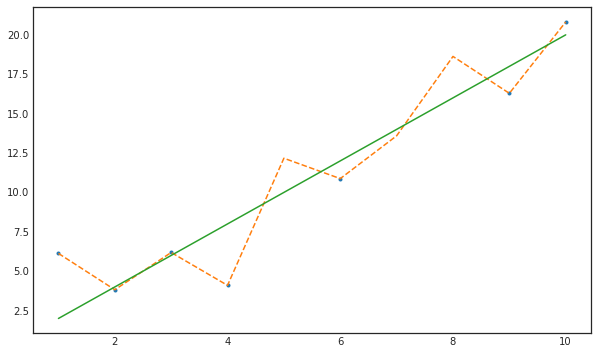
# y_miss_impu = pd.DataFrame(y_miss).interpolate(method='nearest')y_miss_impu = y_miss.copy()y_miss_impu[miss_num] = 0y_miss_impu[miss_num]array([0., 0., 0.])y_miss_impuarray([ 6.12811141, 3.82364263, 6.18746759, 4.10148214, 0. ,
10.87544587, 0. , 0. , 16.28875319, 20.81690097])with plt.style.context('seaborn-white'):
plt.figure(figsize=(10,6))
plt.plot(x,y_miss_impu,'.')
plt.plot(x,y,'--')
plt.plot(x,y_true)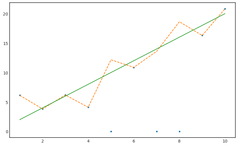
\[\hat{\beta} = \frac{\sum^n_{i=1} y_i x_i}{\sum^n_{i=1} x_i^2}\]
\[\hat{\beta} = \frac{\sum_{i=1}^m y_i x_i + \hat{\beta}_m \sum_{i=m+1}^n x_i^2}{\sum_{i=1}^n x_i^2}\]
y_miss_impuarray([ 6.12811141, 3.82364263, 6.18746759, 4.10148214, 0. ,
10.87544587, 0. , 0. , 16.28875319, 20.81690097])yx_sq = np.sum(y_miss_impu * x);yx_sq468.7641916362335x_sq = sum(x**2);x_sq385beta_hat = yx_sq/x_sqbeta_hat1.2175693289252818y_iter_zero = beta_hat * xy_iter_zeroarray([ 1.21756933, 2.43513866, 3.65270799, 4.87027732, 6.08784664,
7.30541597, 8.5229853 , 9.74055463, 10.95812396, 12.17569329])y_miss_impu_zero = y_miss_impu.copy()y_miss_impu_zero[miss_num] = y_iter_zero[miss_num]y_miss_impu_zeroarray([ 6.12811141, 3.82364263, 6.18746759, 4.10148214, 6.08784664,
10.87544587, 8.5229853 , 9.74055463, 16.28875319, 20.81690097])with plt.style.context('seaborn-white'):
plt.figure(figsize=(10,6))
plt.plot(x,y_miss_impu_zero,'.')
plt.plot(x,y,'--')
plt.plot(x,y_true)
yx_sq_one = sum([y_miss_impu_zero.tolist()] * x);yx_sq_onearray([ 6.12811141, 7.64728526, 18.56240277, 16.40592856,
30.43923322, 65.25267524, 59.66089712, 77.92443705,
146.59877874, 208.16900966])beta_hat_iter_one = yx_sq_one/x_sqbeta_hat_iter_one = (beta_hat + beta_hat_iter_one).mean()y_iter_one = beta_hat_iter_one * xy_iter_onearray([ 1.38296901, 2.76593801, 4.14890702, 5.53187603, 6.91484503,
8.29781404, 9.68078305, 11.06375205, 12.44672106, 13.82969007])y_iter_one[miss_num]array([ 6.91484503, 9.68078305, 11.06375205])y_miss_impu_one = y_miss_impu_zero.copy()y_miss_impu_one[miss_num] = y_iter_one[miss_num]with plt.style.context('seaborn-white'):
plt.figure(figsize=(10,6))
plt.plot(x,y_miss_impu_one,'.')
plt.plot(x,y,'--')
plt.plot(x,y_true)
yx_sq_iter_two = sum([y_miss_impu_one.tolist()] * x);yx_sq_iter_twoarray([ 6.12811141, 7.64728526, 18.56240277, 16.40592856,
34.57422516, 65.25267524, 67.76548132, 88.51001642,
146.59877874, 208.16900966])beta_hat_iter_two = yx_sq_iter_two/x_sqbeta_hat_iter_two = (beta_hat_iter_one + beta_hat_iter_two).mean()y_iter_two = beta_hat_iter_two * xy_iter_two[miss_num]array([ 7.77148648, 10.88008107, 12.43437837])y_miss_impu_two = y_miss_impu_one.copy()y_miss_impu_two[miss_num,] = y_iter_two[miss_num,]with plt.style.context('seaborn-white'):
plt.figure(figsize=(10,6))
plt.plot(x,y_miss_impu_two,'.')
plt.plot(x,y,'--')
plt.plot(x,y_true)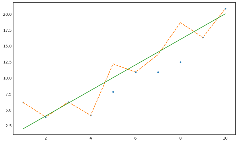
yx_sq_iter_tre = sum([y_iter_two.tolist()] * x);yx_sq_iter_trearray([ 1.5542973 , 6.21718918, 13.98867566, 24.86875674,
38.8574324 , 55.95470266, 76.16056751, 99.47502695,
125.89808098, 155.42972961])beta_hat_iter_tre = yx_sq_iter_tre/x_sqbeta_hat_iter_tre = (beta_hat_iter_two + beta_hat_iter_tre).mean()y_iter_tre = beta_hat_iter_tre * xy_iter_tre[miss_num]array([ 8.54863513, 11.96808918, 13.67781621])y_miss_impu_tre = y_miss_impu_two.copy()y_miss_impu_tre[miss_num] = y_iter_tre[miss_num]with plt.style.context('seaborn-white'):
plt.figure(figsize=(10,6))
plt.plot(x,y_miss_impu_tre,'.')
plt.plot(x,y,'--')
plt.plot(x,y_true)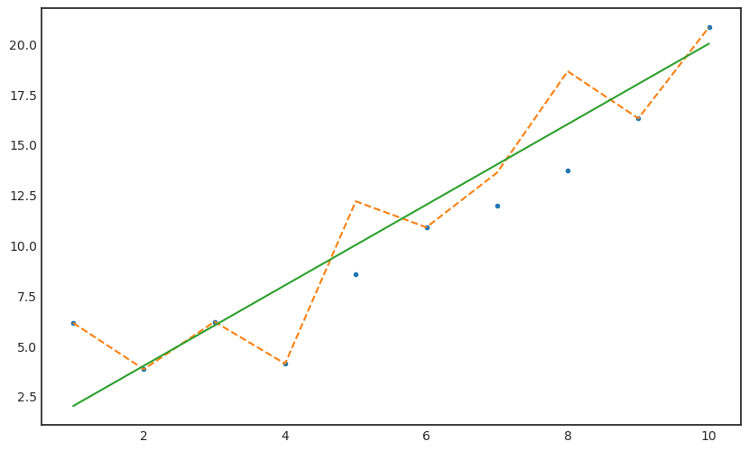
yx_sq_iter_fth = sum([y_iter_tre.tolist()] * x);yx_sq_iter_ftharray([ 1.70972703, 6.8389081 , 15.38754323, 27.35563241,
42.74317564, 61.55017293, 83.77662426, 109.42252964,
138.48788908, 170.97270257])beta_hat_iter_fth = yx_sq_iter_fth/x_sqbeta_hat_iter_fth = (beta_hat_iter_tre + beta_hat_iter_fth).mean()y_iter_fth = beta_hat_iter_fth * xy_iter_fth[miss_num]array([ 9.40349864, 13.1648981 , 15.04559783])y_miss_impu_fth = y_miss_impu_tre.copy()y_miss_impu_fth[miss_num,] = y_iter_fth[miss_num,]with plt.style.context('seaborn-white'):
plt.figure(figsize=(10,6))
plt.plot(x,y_miss_impu_fth,'.')
plt.plot(x,y,'--')
plt.plot(x,y_true)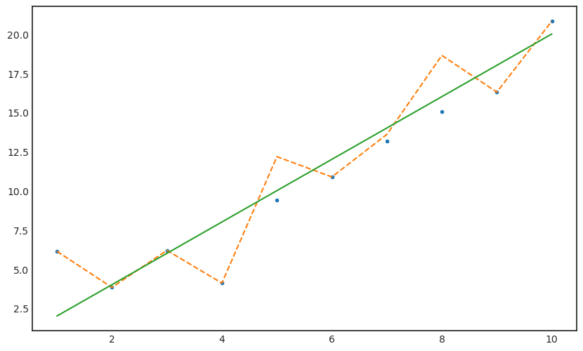
yx_sq_iter_fif = sum([y_iter_fth.tolist()] * x);yx_sq_iter_fifarray([ 1.88069973, 7.52279891, 16.92629755, 30.09119565,
47.01749321, 67.70519022, 92.15428669, 120.36478261,
152.33667799, 188.06997283])beta_hat_iter_fif = yx_sq_iter_fif/x_sqbeta_hat_iter_fif = (beta_hat_iter_fth + beta_hat_iter_fif).mean()y_iter_fif = beta_hat_iter_fif * xy_iter_fif[miss_num]array([10.34384851, 14.48138791, 16.55015761])y_miss_impu_fif = y_miss_impu_fth.copy()y_miss_impu_fif[miss_num] = y_iter_fif[miss_num]with plt.style.context('seaborn-white'):
plt.figure(figsize=(10,6))
plt.plot(x,y_miss_impu_fif,'.')
plt.plot(x,y,'--')
plt.plot(x,y_true)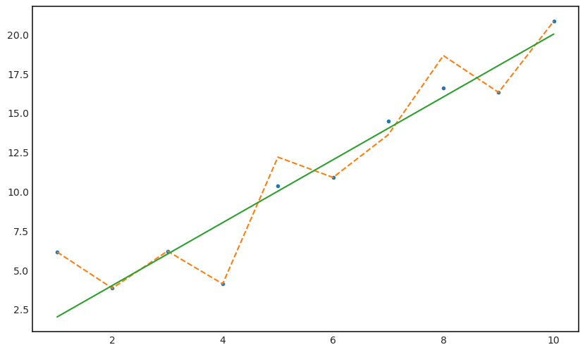
Result
miss_num_1 = [5,7,8]with plt.style.context('seaborn-white'):
fig, ax = plt.subplots(figsize=(20,10))
# fig.suptitle('Figure',fontsize=40)
plt.tight_layout()
ax.plot(x,y_miss,'o',label='Incomplete Data',markersize=8)
ax.plot(x,y,'--',color='blue')
ax.plot(x,y_true,label='True',color='black',alpha=0.5)
ax.plot(miss_num_1,y_miss_impu[miss_num],'o',color='C3',markersize=8)
ax.plot(miss_num_1,y_miss_impu_zero[miss_num],'*',color='C3',markersize=8)
ax.plot(miss_num_1,y_miss_impu_one[miss_num],'*',color='C3',markersize=8)
ax.plot(miss_num_1,y_miss_impu_two[miss_num],'*',color='C3',markersize=8)
ax.plot(miss_num_1,y_miss_impu_tre[miss_num],'*',color='C3',markersize=8)
ax.plot(miss_num_1,y_miss_impu_fth[miss_num],'*',color='C3',markersize=8)
ax.plot(miss_num_1,y_miss_impu_fif[miss_num],'o',color='C3',markersize=8)
ax.legend(fontsize=20,loc='upper left',facecolor='white', frameon=True)
# ax.annotate('1st value',xy=(miss_num[0]+0.1,y_miss_impu[miss_num][0]),fontsize=20)
# ax.annotate('1st value',xy=(miss_num[1]+0.1,y_miss_impu[miss_num][1]),fontsize=20)
# ax.annotate('1st value',xy=(miss_num[2]+0.1,y_miss_impu[miss_num][2]),fontsize=20)
# ax.annotate('5th iteration',xy=(miss_num[0]+0.1,y_miss_impu_fif[miss_num][0]),fontsize=20)
# ax.annotate('5th iteration',xy=(miss_num[1]+0.1,y_miss_impu_fif[miss_num][1]),fontsize=20)
# ax.annotate('5th iteration',xy=(miss_num[2]+0.1,y_miss_impu_fif[miss_num][2]),fontsize=20)
# ax.arrow(miss_num[0]+0.4, y_miss_impu[miss_num][0]+0.6, 0, y_miss_impu_fif[miss_num][0]-1.5,linestyle= 'dashed', head_width=0.1, head_length=0.3, fc='black',ec='black',alpha=0.5)
# ax.arrow(miss_num[1]+0.4, y_miss_impu[miss_num][1]+0.6, 0, y_miss_impu_fif[miss_num][1]-1.5,linestyle= 'dashed', head_width=0.1, head_length=0.3, fc='black',ec='black',alpha=0.5)
# ax.arrow(miss_num[2]+0.4, y_miss_impu[miss_num][2]+0.6, 0, y_miss_impu_fif[miss_num][2]-1.5,linestyle= 'dashed', head_width=0.1, head_length=0.3, fc='black',ec='black',alpha=0.5)
# ax.plot(miss_num, y_miss_impu[miss_num], 'o', markersize=30, markerfacecolor='none', markeredgecolor='red',markeredgewidth=1,color='C4')
ax.tick_params(axis='y', labelsize=20)
ax.tick_params(axis='x', labelsize=20)
# plt.savefig('Self_consistency_Toy.png')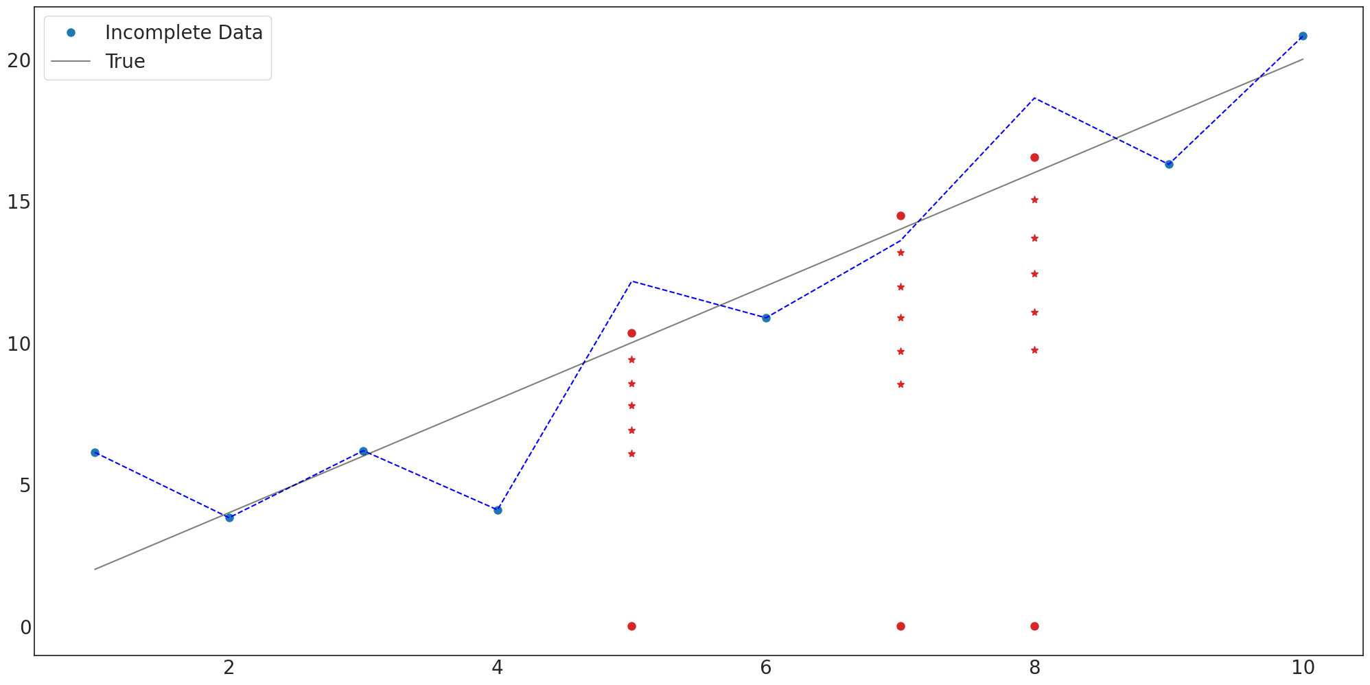
with plt.style.context('seaborn-white'):
    fig, ax = plt.subplots(figsize=(20,10))
    # fig.suptitle('Figure',fontsize=40)
    plt.tight_layout()

    ax.plot(x,y_true,label='True',color='black',alpha=0.5)
    ax.plot(x,y_miss,'o',label='$x_{obs}$',markersize=8)
    # ax.plot(x,y,'--',color='blue')

    # ax.plot(x,y_iter_zero)
    # ax.plot(x,y_iter_one)
    # ax.plot(x,y_iter_two)
    # ax.plot(x,y_iter_tre)
    ax.plot(x,y_iter_fth,color='blue',alpha=0.5,label='$\hat{f}_{obs}$')
    # ax.plot(x,y_iter_fif)
    ax.plot(miss_num_1,y_miss_impu[miss_num],'o',color='C3',markersize=8)
    ax.plot(miss_num_1,y_miss_impu_zero[miss_num],'*',color='C3',markersize=8)
    ax.plot(miss_num_1,y_miss_impu_one[miss_num],'*',color='C3',markersize=8)
    ax.plot(miss_num_1,y_miss_impu_two[miss_num],'*',color='C3',markersize=8)
    ax.plot(miss_num_1,y_miss_impu_tre[miss_num],'*',color='C3',markersize=8)
    ax.plot(miss_num_1,y_miss_impu_fth[miss_num],'o',color='C3',markersize=8)
    # ax.plot(miss_num,y_miss_impu_fif[miss_num],'o',color='C3',markersize=8)

    ax.legend(fontsize=20,loc='upper left',facecolor='white', frameon=True)

    ax.annotate('1st value',xy=(miss_num_1[0]+0.1,y_miss_impu[miss_num][0]),fontsize=20)
    ax.annotate('1st value',xy=(miss_num_1[1]+0.1,y_miss_impu[miss_num][1]),fontsize=20)
    ax.annotate('1st value',xy=(miss_num_1[2]+0.1,y_miss_impu[miss_num][2]),fontsize=20)
    ax.annotate('5th iteration',xy=(miss_num_1[0]+0.1,y_miss_impu_fth[miss_num][0]-0.3),fontsize=20)
    ax.annotate('5th iteration',xy=(miss_num_1[1]+0.1,y_miss_impu_fth[miss_num][1]-0.3),fontsize=20)
    ax.annotate('5th iteration',xy=(miss_num_1[2]+0.1,y_miss_impu_fth[miss_num][2]-0.3),fontsize=20)

    ax.arrow(miss_num_1[0]+0.4, y_miss_impu[miss_num][0]+0.6, 0, y_miss_impu_fth[miss_num][0]-1.5,linestyle= 'dashed', head_width=0.1, head_length=0.3, fc='black',ec='black',alpha=0.5)
    ax.arrow(miss_num_1[1]+0.4, y_miss_impu[miss_num][1]+0.6, 0, y_miss_impu_fth[miss_num][1]-1.5,linestyle= 'dashed', head_width=0.1, head_length=0.3, fc='black',ec='black',alpha=0.5)
    ax.arrow(miss_num_1[2]+0.4, y_miss_impu[miss_num][2]+0.6, 0, y_miss_impu_fth[miss_num][2]-1.5,linestyle= 'dashed', head_width=0.1, head_length=0.3, fc='black',ec='black',alpha=0.5)

    # ax.plot(miss_num_1, y_miss_impu[miss_num], 'o', markersize=30, markerfacecolor='none', markeredgecolor='red',markeredgewidth=1,color='C4')

    ax.tick_params(axis='y', labelsize=20)
    ax.tick_params(axis='x', labelsize=20)
# plt.savefig('Self_consistency_Toy_0617.png')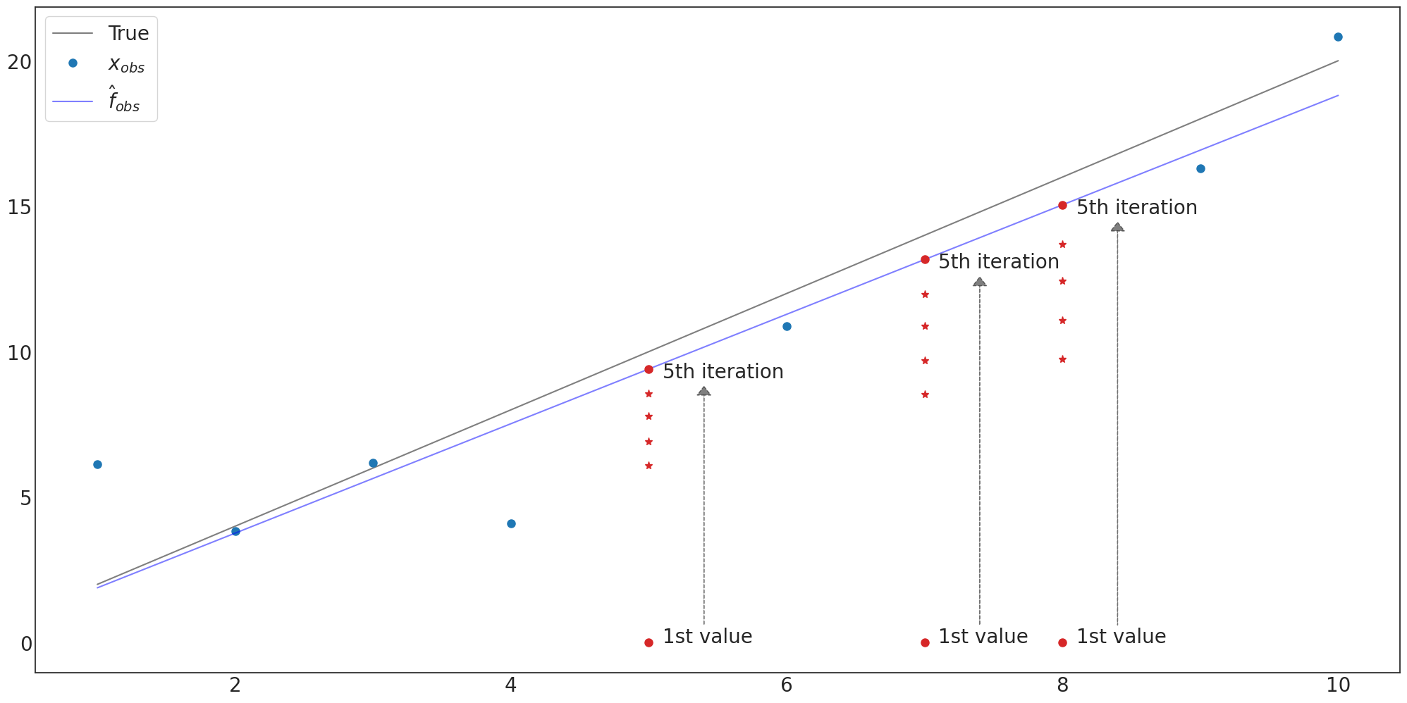
Figure on frequency
T = 500

t = np.arange(T)/T * 10

y_true = 3*np.sin(0.5*t) + 1.2*np.sin(1.0*t) + 0.5*np.sin(1.2*t)

y = y_true + np.random.normal(size=T)plt.figure(figsize=(20,10))
plt.plot(t,y_true,color='red',label = 'true')
plt.plot(t,y,'',color='black',label = 'f')
plt.legend(fontsize=15,loc='lower left',facecolor='white', frameon=True)
# plt.savefig('1.png')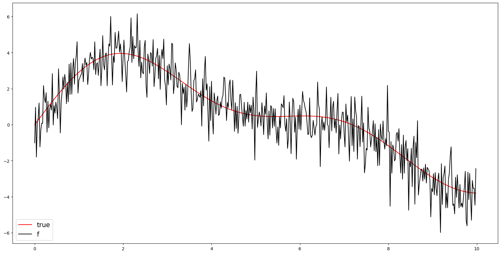
random_num = np.random.choice(range(500), size=400, replace=False)y[random_num] = np.nanplt.figure(figsize=(20,10))
plt.plot(t,y_true,color='red',label = 'true')
plt.plot(t,y,'.',color='black',label = 'f')
plt.legend(fontsize=15,loc='lower left',facecolor='white', frameon=True)
# plt.savefig('1.png')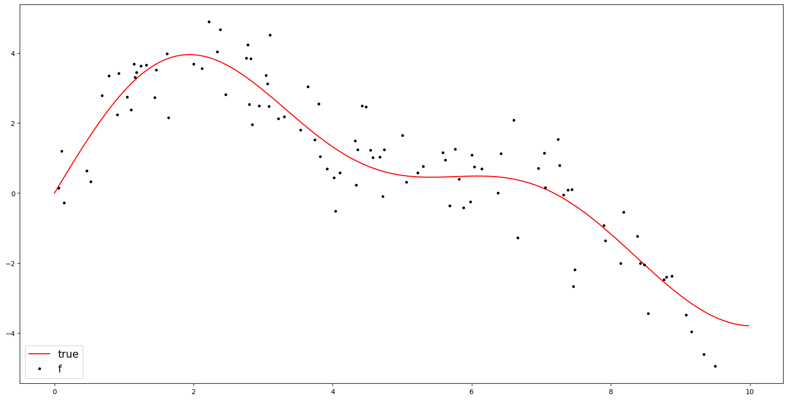
y[random_num] = 0plt.figure(figsize=(20,10))
plt.plot(t,y_true,color='red',label = 'true')
plt.plot(t,y,'.',color='black',label = 'f')
plt.legend(fontsize=15,loc='lower left',facecolor='white', frameon=True)
# plt.savefig('1.png')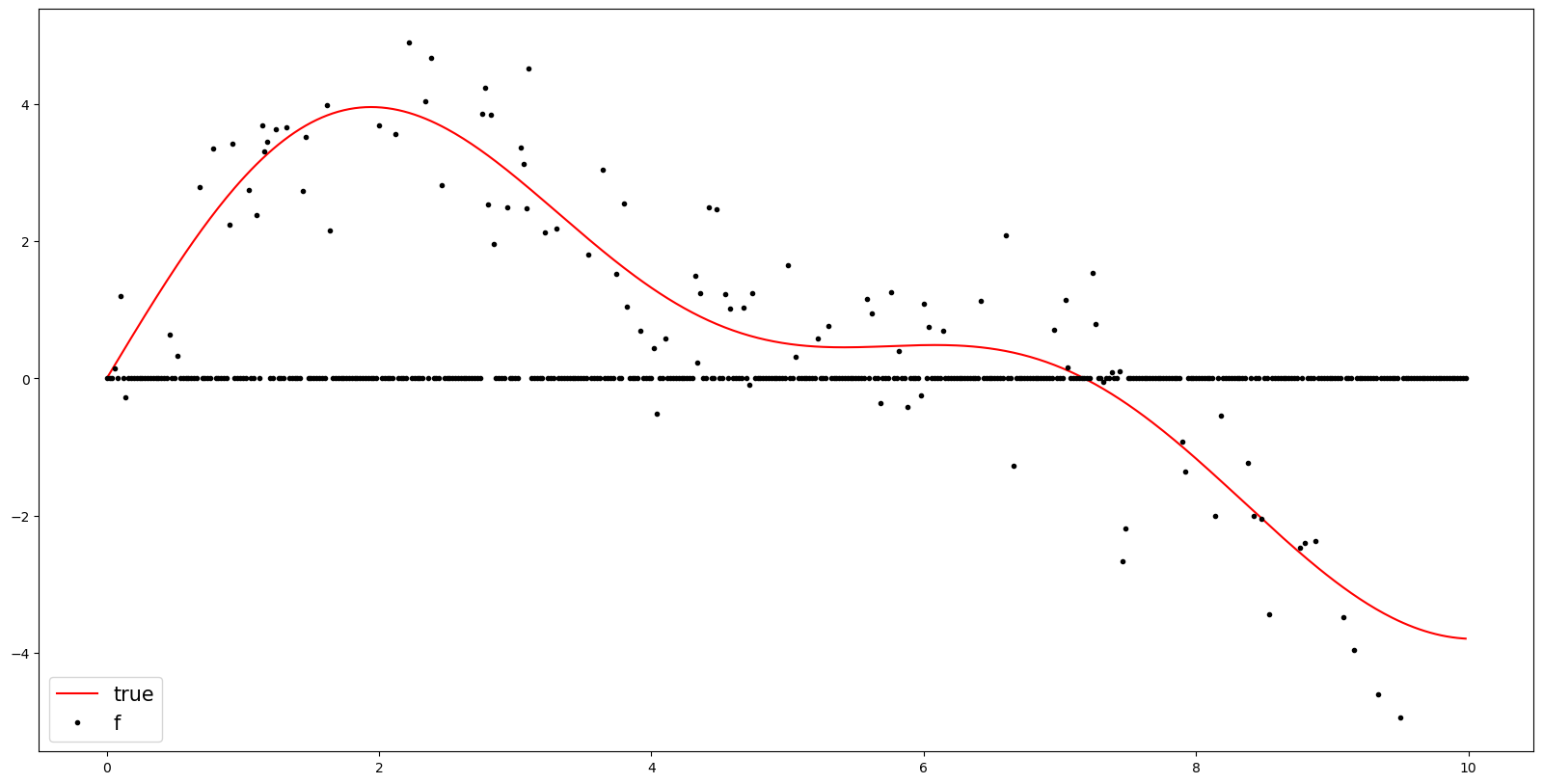
y_inter = pd.DataFrame(y).interpolate(method='linear').fillna(method='bfill').fillna(method='ffill').to_numpy().tolist()plt.figure(figsize=(20,10))
plt.plot(t,y_true,color='red',label = 'true')
plt.plot(t,y,'.',color='black',label = 'f')
plt.plot(t,y_inter,color = 'blue')
plt.legend(fontsize=15,loc='lower left',facecolor='white', frameon=True)
# plt.savefig('1.png')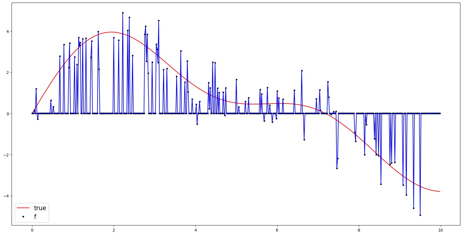
np.array(y_inter).reshape(-1)[random_num]array([0., 0., 0., 0., 0., 0., 0., 0., 0., 0., 0., 0., 0., 0., 0., 0., 0.,
0., 0., 0., 0., 0., 0., 0., 0., 0., 0., 0., 0., 0., 0., 0., 0., 0.,
0., 0., 0., 0., 0., 0., 0., 0., 0., 0., 0., 0., 0., 0., 0., 0., 0.,
0., 0., 0., 0., 0., 0., 0., 0., 0., 0., 0., 0., 0., 0., 0., 0., 0.,
0., 0., 0., 0., 0., 0., 0., 0., 0., 0., 0., 0., 0., 0., 0., 0., 0.,
0., 0., 0., 0., 0., 0., 0., 0., 0., 0., 0., 0., 0., 0., 0., 0., 0.,
0., 0., 0., 0., 0., 0., 0., 0., 0., 0., 0., 0., 0., 0., 0., 0., 0.,
0., 0., 0., 0., 0., 0., 0., 0., 0., 0., 0., 0., 0., 0., 0., 0., 0.,
0., 0., 0., 0., 0., 0., 0., 0., 0., 0., 0., 0., 0., 0., 0., 0., 0.,
0., 0., 0., 0., 0., 0., 0., 0., 0., 0., 0., 0., 0., 0., 0., 0., 0.,
0., 0., 0., 0., 0., 0., 0., 0., 0., 0., 0., 0., 0., 0., 0., 0., 0.,
0., 0., 0., 0., 0., 0., 0., 0., 0., 0., 0., 0., 0., 0., 0., 0., 0.,
0., 0., 0., 0., 0., 0., 0., 0., 0., 0., 0., 0., 0., 0., 0., 0., 0.,
0., 0., 0., 0., 0., 0., 0., 0., 0., 0., 0., 0., 0., 0., 0., 0., 0.,
0., 0., 0., 0., 0., 0., 0., 0., 0., 0., 0., 0., 0., 0., 0., 0., 0.,
0., 0., 0., 0., 0., 0., 0., 0., 0., 0., 0., 0., 0., 0., 0., 0., 0.,
0., 0., 0., 0., 0., 0., 0., 0., 0., 0., 0., 0., 0., 0., 0., 0., 0.,
0., 0., 0., 0., 0., 0., 0., 0., 0., 0., 0., 0., 0., 0., 0., 0., 0.,
0., 0., 0., 0., 0., 0., 0., 0., 0., 0., 0., 0., 0., 0., 0., 0., 0.,
0., 0., 0., 0., 0., 0., 0., 0., 0., 0., 0., 0., 0., 0., 0., 0., 0.,
0., 0., 0., 0., 0., 0., 0., 0., 0., 0., 0., 0., 0., 0., 0., 0., 0.,
0., 0., 0., 0., 0., 0., 0., 0., 0., 0., 0., 0., 0., 0., 0., 0., 0.,
0., 0., 0., 0., 0., 0., 0., 0., 0., 0., 0., 0., 0., 0., 0., 0., 0.,
0., 0., 0., 0., 0., 0., 0., 0., 0.])import tensorflow as tf
from tensorflow.keras.models import Sequential
from tensorflow.keras.layers import LSTM, Dense# Define the number of time steps for the LSTM model
time_steps = 10
# Create input and output sequences by shifting the data
X = []
Y = []
for i in range(len(y) - time_steps):
X.append(y[i:i+time_steps])
Y.append(y[i+time_steps])
# Convert the sequences to numpy arrays
X = np.array(X)
Y = np.array(Y)
# Reshape the input data to match the LSTM input shape
X = np.reshape(X, (X.shape[0], X.shape[1], 1))# Define the LSTM model
model = Sequential()
model.add(LSTM(32, input_shape=(time_steps, 1)))
model.add(Dense(1))
# Compile the model
model.compile(loss='mean_squared_error', optimizer='adam')
# Train the model
model.fit(X, Y, epochs=1, batch_size=32)16/16 [==============================] - 2s 5ms/step - loss: 1.0766<keras.callbacks.History at 0x7fa83818bdf0>np.array(Y).reshape(-1)[random_num]IndexError: index 492 is out of bounds for axis 0 with size 490plt.plot(t[:490],Y)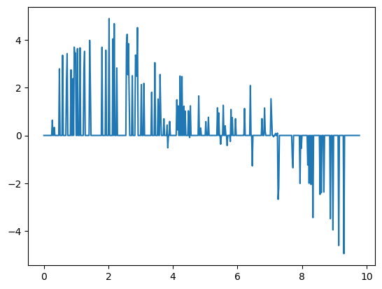
Footnotes
확률 과정 중 과거의 정보를 알고 있다면 미래의 기댓값이 현재값과 동일한 과정↩︎